ST03N versus STAD: Aggregate workload or one SAP execution?
A manufacturer's transaction average looks acceptable while a small group of production users experiences severe delays.

Source review:
START HERE · NO PRIOR TOPIC KNOWLEDGE NEEDED
What it is. Why it matters.
Workload statistics describe how SAP tasks use time and resources. ST03N supports aggregated analysis; STAD helps examine individual statistical records in the relevant context.
Completely new to SAP?
Manufacturers use SAP to connect work such as buying components, recording inventory, planning production, shipping equipment and accounting for costs. SAP S/4HANA is an enterprise resource planning system: it connects these activities through shared business data.
SAP Basis work keeps relevant SAP systems running. Logs, background jobs and connection tools help explain what happened to a task at a particular time.
A transaction code, or t-code, is a shortcut to a task in classic SAP GUI. Fiori apps provide another way to work. Names and screens depend on the product and release; you do not need a live system to learn the concepts in this guide.

Scope and source-review notes
Scope and evidence
Source review by FAST SAP SOLUTIONS® editorial. This badge describes our editorial review; it does not represent SAP certification or independent endorsement.
Classic AS ABAP ST03N workload and STAD statistical-record analysis for performance support. Available detail, retention, collector operation and timing fields vary by release and setup; statistical records are not a full browser or business-process trace.
Documentation review on 14 November 2026 used the available official SAP indexed excerpts; several SAP Help pages returned no readable full text. The worked case and proposed checks are original illustrative teaching material, not execution evidence from a customer SAP system. Exact fields, permitted actions and behavior must be confirmed against the installed product, release and configuration.
A MANUFACTURING EXAMPLE
Find the slow requests behind a plant average
An average can hide slow executions
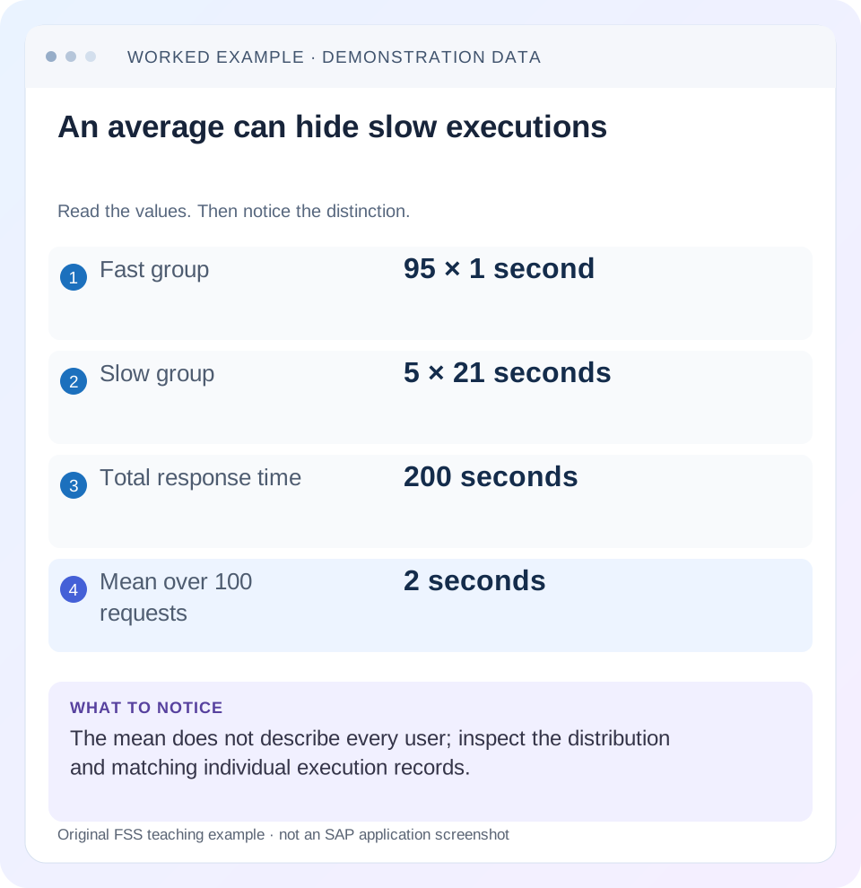
Read the example values
- Fast group
- 95 × 1 second
- Slow group
- 5 × 21 seconds
- Total response time
- 200 seconds
- Mean over 100 requests
- 2 seconds
Words you’ll meet in this guide
- Instance
- A running SAP application-server environment.
- Client
- A logically separate data and configuration context in an ABAP system.
- Log
- A recorded sequence of events and messages.
- ABAP
- SAP’s programming language for business applications.
- Fiori
- SAP’s approach to business application design.
- GUI
- Graphical user interface. SAP GUI is a desktop interface used for many classic SAP tasks.
- HTTP
- The request-and-response protocol used by web applications and APIs.
- SQL
- A language used to read and work with database data.
Preview the practical steps
SEE THE CONNECTION
See it in a simple example.
A small example to make the idea concrete.
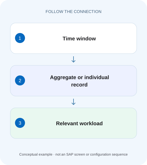
Find the slow requests behind a plant average
A manufacturer's transaction average looks acceptable while a small group of production users experiences severe delays.
Choose the question before the monitor
Use ST03N to investigate workload patterns across a selected population and period.
Audience and prerequisites
This lesson is for Basis and performance analysts with permitted access to workload and statistical records.
Worked dataset: the average hides five bad requests
Our fictional transaction population contains 100 comparable executions in one hour.
Find the slow requests behind a plant average
A manufacturer's transaction average looks acceptable while a small group of production users experiences severe delays.
Compare aggregate workload with the relevant single-request evidence before deciding which users and execution paths are affected.
| Reader | Business question | Evidence to carry forward |
|---|---|---|
| SAP developers and application teams supporting manufacturers | Find the slow requests behind a plant average | Compare aggregate workload with the relevant single-request evidence before deciding which users and execution paths are affected. |
01 Choose the question before the monitor
Use ST03N to investigate workload patterns across a selected population and period. Use STAD to investigate retained statistical evidence for a particular execution or dialog step. The two views complement each other: aggregates show patterns, while individual records help explain which executions contributed to them.
SAP documents STAD's detailed resource and response-time analysis and ST03N's aggregated presentation. A transaction average cannot prove that every user had the same experience. Likewise, one slow execution cannot establish that the whole system or an entire day was slow. Define the population behind every performance statement. [2] [3]
02 Audience and prerequisites
This lesson is for Basis and performance analysts with permitted access to workload and statistical records. Obtain the system, incident time and time zone, user or technical identity, transaction/request context and relevant instance where known. Establish available retention and collector health before promising to recover a historical execution.
The examples use classic AS ABAP monitoring concepts. A Fiori click can involve browser work, HTTP calls, backend steps and remote systems; no single ABAP record automatically represents that entire user experience. Installed-release fields and collection settings determine what you can observe. Keep frontend elapsed time and backend statistical time distinct when comparing measurements.
03 Worked dataset: the average hides five bad requests
Our fictional transaction population contains 100 comparable executions in one hour. Ninety-five take one second each and five take 21 seconds each. Total response time is 95 plus 105, or 200 seconds; the average is two seconds. Most executions are faster than that average, while five users experience a much larger delay.
Suppose the five slow requests share one instance and a broad document selection. The aggregate identifies an investigation opportunity, but the shared cause remains unproven. You need individual records and input context to distinguish instance pressure, greater selected work and some other coincident behavior. All timings are invented for arithmetic practice.
| Group | Count | Time each | Total |
|---|---|---|---|
| Fast executions | 95 | 1 s | 95 s |
| Slow executions | 5 | 21 s | 105 s |
| Combined | 100 | 2 s mean | 200 s |
04 Establish a reproducible ST03N population
Record the selected system/instance scope, period, task type and transaction or workload category. Compare the same view definitions when discussing averages. A dialog-only view and a mixed dialog/background population answer different questions even if both are labeled with the same day.
Inspect response-time distribution where available, execution counts and total workload as well as the average. SAP's workload documentation explicitly includes response-time distribution statistics. In the example, identifying the five 21-second requests is more useful than declaring the two-second mean acceptable or unacceptable without the business expectation and tail behavior. [1]
05 Weight averages by execution count
Do not average averages from groups of different sizes. Imagine instance A has 90 requests averaging one second, while B has 10 averaging 11 seconds. The combined average is (90 × 1 + 10 × 11) / 100 = two seconds, not six seconds.
Retain counts and totals when comparing periods or instances. A lower average after a change can result from more cheap requests rather than improvement of the expensive path. Conversely, total workload can increase because volume grew while per-request performance stayed stable. These are different operational stories, and the denominator determines which story is supported.
A: 90 executions × 1 second = 90 seconds
B: 10 executions × 11 seconds = 110 seconds
Combined mean = (90 + 110) / (90 + 10) = 2 seconds
Unweighted mean of 1 and 11 = 6 seconds: wrong population weighting.
06 Find the relevant STAD record
Select a focused interval around the reported action and narrow by the supported user, transaction or instance criteria. Confirm the time convention and expected technical identity. An interface or HTTP action may execute under a service user, so searching only the employee's GUI identity can miss the relevant backend record.
Match records to the actual action and step. A multi-step transaction can produce several records, and a user may execute the same action repeatedly. Use timestamps and available correlation context to distinguish the 10:05 failure from a 10:08 successful retry. Missing retained records are an evidence gap, not proof that the request never ran. [2]
07 Read timing components as diagnostic directions
Inspect the documented response-time components for the relevant task and release. Components such as CPU, database processing, wait or remote-call-related information can guide the next investigation, but they should be interpreted using their precise definitions. Do not add overlapping fields or invent an equality from labels alone.
For a fictional slow record with high database-related time, a targeted database/SQL investigation is a reasonable next step. It is not yet evidence of a particular missing index. If host CPU is high during the same interval, correlate the correct host and processes. If the backend record is fast but the user waits, inspect the rest of the route and frontend timing.
08 Relate the slow record to business input
Compare the selected data volume and process state with a representative fast execution. An order display for one item and a report spanning twelve months are not equivalent workloads merely because they share a transaction or program. Record the input dimensions that can affect work: date range, organization, object count and relevant mode.
For the five slow requests, test whether the broad selection explains greater database work. If all slow requests ran on B but only B received the broad selections, instance and input effects are confounded. Obtain a controlled comparison or a sufficiently detailed record before assigning the cause to B's configuration.
09 Design a focused next measurement
Choose the smallest measurement that resolves the leading uncertainty. A SQL-heavy record can justify an authorized targeted SQL trace or analysis of the corresponding statement. An execution waiting on another system requires correlation with that remote route and request. A workload pattern concentrated at a scheduled batch window suggests reviewing jobs and competing resources.
Define the question, interval, identity and stop condition before tracing. The useful output is a connection between the statistical symptom and a specific expensive or waiting operation. Capturing broad traces without a reproduction or hypothesis can create large sensitive datasets while still failing to identify the relevant request.
10 Troubleshoot misleading comparisons
If ST03N looks normal while one user complains, inspect distribution and the user's actual request. If STAD has no matching record, check retention, timestamp, task type, technical identity and instance scope. If a repeated request is faster, consider warm-up, caching, changed data and reduced selection before crediting a code change.
If totals differ between two analysts, compare selections and view definitions first. One may include all instances and another only the local instance. One may inspect a completed daily aggregate while another uses a partial interval. Agreement on labels is not agreement on the underlying population; preserve the actual selection criteria in the incident.
| Observation | Next check |
|---|---|
| Normal mean, isolated complaint | Distribution and matching execution |
| No individual record | Retention, task, time and identity |
| High DB-related time | Relevant statement and selected work |
| Fast backend, slow browser | Other calls, network and frontend timing |
| Lower mean after filtering | Counts and excluded expensive path |
11 Verify with comparable positive and boundary checks
For the dataset exercise, calculate the two-second mean and identify the five slow records. Then remove the five slow requests: the mean becomes one second, but the original bad path has not been improved; it has been excluded. This negative comparison tests whether the analyst can distinguish selection change from performance change.
For an approved correction, compare equivalent input, workload period and instance context, record actual timings and inspect whether the slow-tail behavior changed. Include a representative unaffected request. A zero-execution period has no meaningful observed transaction average, and a single successful repeat is insufficient for a system-wide improvement claim. State the size and limits of the measured sample.
12 Build a handoff from population to execution
A useful report connects four things: the original user symptom, the aggregate population, the matching individual record and the next hypothesis. For example: “100 executions, mean two seconds; five 21-second executions on B with broad date ranges; matching record shows database-related time; need statement-level evidence for that selection.”
Attach sanitized record references and reproducible selection criteria. Keep invented teaching data out of real incident conclusions. After the next measurement, revise the hypothesis to match the evidence rather than preserving the first guess. A performance investigation progresses by reducing uncertainty, not by accumulating monitor screenshots.
Before publishing a before-and-after claim, write the comparison as a small experimental statement: same report selection, same relevant task type, known instance scope and stated execution count. Record what changed besides the proposed correction, such as data volume or competing batch activity. If those conditions cannot be aligned, report an observational comparison with its limits. That is still useful evidence, but it cannot support a precise causal improvement claim.
For workload growth, compare two fictional days with identical one-second executions but 100 requests on day 1 and 1,000 on day 2. Total response-time workload grows from 100 to 1,000 seconds while mean per execution stays one second. That is volume growth, not a tenfold per-request regression. Reverse the comparison by holding count constant while duration grows, and the performance question changes. Retaining both count and duration prevents a capacity discussion from being confused with inefficient code and helps explain why total CPU/database demand can increase even when the representative user request has not slowed.
13 Questions that prevent overclaiming
Does STAD explain an entire order-to-cash process? It analyzes relevant execution records and steps; the business process may span many such records and systems. Can ST03N prove a particular SQL statement is defective? No; it helps locate the workload requiring more precise evidence.
Should an average be ignored? No. It is useful when its population, count and distribution are understood. Can two requests with the same transaction code be compared directly? Only after relevant input and context are aligned. Continue with work-process, host-resource and job analysis when those layers explain the timing pattern suggested by the statistics.
Related services and next steps
Primary sources
Found this useful?
Share this guide with your network, or leave a like.
Your like is saved in this browser.